The budget line formula shows all possible combinations of goods that consumers can purchase if exhausted their entire budget on such property.
Consumer Decision
The decision of the consumer as to the set of goods they want to purchase for consumption is determined by two factors:
- Tastes or preferences
- Rent Available
Basic Assumptions
Consumer theory begins with three basic assumptions about people’s preferences:
- Complete Preferences: Consumers can compare and order according to your preference. It is layers of deciding which prefers and is indifferent (proposals that will satisfy you equally)
- Preferences Transitive (transitivity): If a consumer prefers the product or product group A to B and B before C, he prefers A to C as well.
- Insatiability: Consumers prefer a larger amount of any good to less.
Available Income
The disposable income sets a limit on the spending capacity of the consumer, who can consume at most the amount of his income.
The budget line formula represents all possible combinations of goods that the consumer can acquire if he exhausts his entire budget.
The Equation of Budget Line Formula
The equation of the budget line formula depends on the income of consumers and the prices of goods.
Marginal Rate of Market Substitution
The marginal rate of substitution Market is the rate at which the consumer can trade one good for another without altering the amount of money spent.
More from Business Study Notes:- Indifference Curve Analysis
Change in Income
Raising incomes by keeping prices constant implies a parallel shift to the right – up the budget line and the budget set is widening. If income is reduced, the budget subtraction shifts left-down and the budget set is smaller. In neither case does the slope change as prices remain constant.
Variations in Product Prices
The rising price of one of the real causes the budget line formula to rotate to the left – down and the budget is set lower. The value of the straight line varies (since the relative price of the two goods changes).
The cut-off point with the axis of that good whose price has not changed remains constant. However, the cut-off point of the goods whose price has increased is close to the origin. If the price of one of the goods is reduced, it causes the budget line to rotate to the right-up. Hence, the budget is set to increase. The value of the line also varies (since the relative price of the two goods changes). When there is a simultaneous variation of prices and income, the budget subtraction shifts and changes the slope and in turn the budget set.
Suppose, the change in the price of the good X is greater than the variation of the good. Then, the slope of the budget line increases. If the change in the price of the good X is less than the variation of the good and the slope of the budget line decreases. If the price of the two goods varies, but in such a way that I did not vary the relation between them. So, there will be a parallel shift of the budget line as its slope does not change. The price changes of the line of budgetary restriction coupled with a change in its slope causes two effects:
- Income effect: The increase in the price of a good causes a negative income effect. Since, it decreases the purchasing power of the income (given a certain level of income can buy less quantity of that good).
- Substitution effect: The price ratio between the two goods contemplated is altered.
Budgetary Restriction – Budget Line
In a delimited period of time, the consumer has a certain amount of money that he can devote to consumption. Your rent can be biweekly, monthly, yearly. Given this amount of money, which we will call R, the subject must decide what goods to consume. We will continue to assume that the choice focuses on only two goods. So, to find out how the money destined for consumption is exhausted. Basically, we need to know, besides the rent, the prices of the goods. The given income and prices, the sets of goods that the consumer can access are given by the following restriction:
(1) p x x + p y y = R
When we study consumer preferences, the proposed model is for the choice between two goods. There we made the proviso that one of the goods is a specific good eg. clothes. Also, the other was a composite good that encompassed the whole Rest of the goods. When we study the budget constraint we maintain this approach, then we can say that the good X is the demand for consumer clothing. Where, the good Y represents everything else that the consumer wants to acquire, in addition to clothing.
It is useful to suppose that the good Y is the money that the consumer can spend on the consumption of other goods. Automatically, we have that the Py will be equal to 1, since the price of a monetary unit is a monetary unit. Then we can write the budget constraint as follows:
(2) P x x + y = R
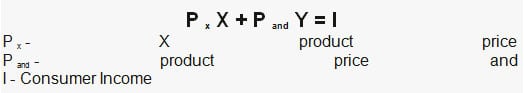
In the two-dimensional space, we can represent this restriction using Figure 1.
There we see all the baskets of goods that are affordable to the consumer, this set is called the budget set. On the thick line are the baskets of goods that deplete the consumer’s budget, and meet the restriction:
(3) p x x + p y = R
If we order formula (3), we can express the budget constraint in such a way as to show the consumption of a good according to the prices. Although, prices include both goods and the quantity consumed of the remaining goods. In this way we have the expression:
(4) Y = R / p – p x / p x
Then, given the prices (Px, Py) and income (R). The budget constraint is drawn as a straight line with negative slope that tells us the relation to which the market replaces the good Y for the good X.
Changes in the Budget Restriction
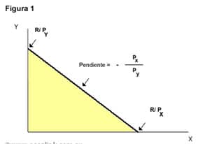
The function presented in the previous section depends on the prices of the goods (Px, Py). The consumer income (R), and then the changes in the function will be a product of changes in these given variables.
If rent (R) is modified, then it is a parallel shift of the budget constraint. If the rent increases the restriction will move to the right, if it contracts, the restriction will shift to the left. This indicates that, given the prices, an increase in consumer income implies that the latter will have the possibility of acquiring more of both goods. If we look at the intercept and the abscissa at the origin, in Figure 2 we see that both are shifted to the right. So, the amount the consumer could purchase good X or Y is greater good in both cases. We must emphasize that the rate at which the two goods are replaced in the market has not changed.
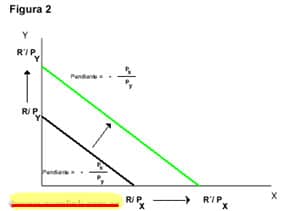
Thus we see in Figure 3 , how the restriction to an increase in the price of good moves X. It can be seen that the intercept is unchanged. However, it decreases the amount that can be purchased for good X if all income is destined to its consumption. For this reason the abscissa in the origin moves towards the left. When prices change, the taste replacement market changes.
Other Considerations – Budget Line
We can think about how the budgetary restriction will be modified in the face of economic policy measures such as taxes, subsidies and rationing.
Taxes
If the tax (or subsidy) is practiced on the amount consumed, the effect is analogous to an increase in price. If per unit of good X that the individual consumes, it must pay the state a certain amount t. Then you are paying Px + t, this is equivalent to an increase in the price of good X and graphically. So, we have seen that implies an increase in the slope of the budget constraint.
The tax is applied on the value of the property , that is, about the price of goods. Thus we have that if the price of good X is Px and a tax on the amount of sales, the price paid by the consumer becomes Px (1+ applies t ). That is, the bidder pays Px and Px * t to the state.
Subsidies
Subsidies on the quantity and value of the asset affect income and prices in a manner analogous to a tax, but in the opposite direction.
Another way to apply a policy can be through a tax (or subsidy) of fixed rate. This means that the State takes a fixed amount of money regardless of the quantities consumed. In graphic terms, this translates into a parallel shift of the budget constraint to the left (to the right if it is a subsidy).
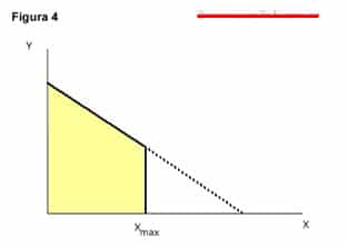
Rationing
Finally, we can name another policy measure known as rationing. The rationing consists of establishing the maximum amount that the individual can acquire. In graphic terms we can see in Figure 4 how the budget set is changed. The individual can consume all those combinations such that the amount of X is less than X max.
Policy Combination
Finally, in Figure 5 we can see a combination of policies. In this case, the individual can consume the good X at the price Px up to the quantity X1 at the price Px. From the quantity X1, if the consumer wishes to increase the quantity purchased of the good X, he must pay the price (Px + t). In this way we see how the budget constraint presents a break at the height of X1. Hence, for quantities greater than X1 the slope of the budget constraint increases, i.e. the good X becomes more expensive than the Y.

Hello everyone! This is Richard Daniels, a full-time passionate researcher & blogger. He holds a Ph.D. degree in Economics. He loves to write about economics, e-commerce, and business-related topics for students to assist them in their studies. That's the sole purpose of Business Study Notes.
Love my efforts? Don't forget to share this blog.


