Modified Internal Rate of Return Analysis: In certain cases, the Internal Rate of Return (IRR) exhibits certain problems which are covered with the new concept of Modified Internal Rate of Return (MIRR).

Modified Internal Rate of Return is a useful technique that uses different methods for calculation of IRR in those cases where there comes a problem with calculation of IRR with the ordinary method of trial & error.
Problems with Internal Rate of Return
There are certain problems that come in the calculation of IRR by using its ordinary method. The following are two important problems in this regard.
- In the case where the project useful life is more than two years.
- When there is the presence of non-normal cash flows or more net cash outflows (in addition to the outflow of initial investment) at a certain point in the future.
The above two cases result in the creation of multiple IRRs which makes the NPV of the project equal to zero.
Example
For example, if Mr. Ali made an initial investment of $ 100 and there are net cash inflows (cash receipts) at the end of the year equal to $ 500. There are also net cash outflows (cash payments) of $ 500 at the end of second year. The cash flow pattern is shown in the below diagram.

There is a cash outflow of $ 100 in the above diagram in year 0. There is a cash inflow of $ 500 represented by an upward arrow in the first year. Moreover, there is a net cash outflow of $ 500 which is represented by a downward arrow in year 2. Following is the calculation of the IRR of this project.
NPV = 0 =-100 + 500/(1+IRR) – 500/(1+IRR)2
By solving through trial & error method
IRR = (approx) 38% & 260%
The solution to the above example results in two values of IRR. Now the question is which value is the correct one. In order to deal with this problem, there is another concept of IRR which is known as Modified Internal Rate of Return (MIRR) in which another method of calculation is used.
Modified Internal Rate of Return (MIRR)
Modified Internal Rate of Return is the cash inflows & cash outflows of each year are separated and a market discount rate “k” is used. When cash inflows & cash outflows are plotted on the diagram, they can be easily separated from each other instead of making their net cash flows.
In the next step all the future cash outflows are discounted back to the present. In the next step of the MIRR, all the cash inflows are compounded to the future end period or project’s end life. The concept of the compounding of cash inflows is based on the assumption that these will be reinvested at the cost of capital.
In the next step, certain rate is used which equalizes the future value of cash inflows with the present value of cash outflows. This equalizing rate is known as the Modified Internal Rate of Return (MIRR). The following is the formula for MIRR.
(1+MIRR)n = Future value of all cash inflows / Present value of all cash outflows
(1+MIRR)n = CF(in) * (1+k)n-t / CF(out)/(1+k)t
In the above equation of MIRR, two discount rates are used. MIRR is the first discount rate while the other is the one is the opportunity cost of capital used in NPV calculation.
Example:
In the above-mentioned example where the initial investment of the project is $ 100. There is a $ 500 net cash inflow in the first year and net cash outflows of $ 500 in the second year. If the ordinary trial & error method of NPV calculation is used then IRR will be
NPV = o = -100 + 500/ (1+IRR) – 500/ (1+IRR)2
The resulting answer gives two values of IRR which are 38% and 260%. These two values of IRR are not correct because the Modified Internal Rate of Return (MIRR) approach should be used to calculate the correct IRR for this project.
By applying the MIRR formula in the example, suppose that the cost of capital k = 10%.
(1+MIRR)n = CF(in) * (1+k)n-t / CF(out)/(1+k)t
The compound factor is 1.10 because it is supposed that the risk-free rate of return = i = 10%. n = total life span of the project while “t” corresponds to the time in which specific cash flow occurs.
(1+MIRR)2 = 500 x (1+0.1)2-1 / (100/1.1) + (500/(1+0.1)2
(1+MIRR)2 = 550 / 513
(1+MIRR)2 = 1.07
MIRR = 0.0344 = 3.44%
The answer obtained from this formula is different from the one obtained with ordinary formula of IRR. But answer provided by the MIRR is more realistic and best one.
NPV Projects with Different Live Spans
Let’s suppose there are two projects having different life spans. Then it is not possible to compare them in an ordinary manner and selection of the project having higher Net Present Value. The reason behind this un-equality is that one project is offering cash flows for a shorter period of time while other is offering cash flows for longer period of time. There are two approaches that are used to compare the projects having different life spans. These two approaches are as follows.
- Common Life Approach
- Equivalent Annual Annuity Approach
Common Life Approach
For making comparisons among two investment opportunities there is an option to equate the life of both projects. For this purpose, the cash flow pattern of each project is repeated over a horizon that equals the least common multiple of the life of two investments.
For example, if there are two projects and the first project’s life is 2 year and the second project’s life is one year than the least common multiple of their lives is two. The cash flow patterns of the second project are repeated for next year so both projects can be compared.
Similarly, if the life of the first project is three years and the life of the second project is two years than the least common multiple of their lives will be six. In this case, the cash flows of the first project are repeated twice & the cash flows of the second project are repeated thrice.
When the lives of both projects are equated then it is easy to calculate & compare the net present value of both projects.
Example:
There are two projects with whose cash flows are as follow
Project A = Io = -$ 200, year1 = +$ 200, year2 =+$200
Project B = Io = -$ 100, year1 = +$ 200
By applying a simple NPV formula (Assumption i = 10%)
Project A = -200 + 200/1.1 + 200/(1.1)2 = +$ 147
Project B = -100 + 200/1.1 = +$82
From the above calculation by using a simple NPV formula, it is concluded that project A is better. But this is not true because in this case comparison is made between oranges & apples based on the difference in the lives of projects.
By applying the correct formula of common life approach
Least Common Multiple = Common Life Span = 2 years
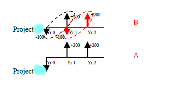
The cash flows pattern of project B is replicated twice so that it can be equal to the life span of project A. There is an outflow of 100 & inflow of 200 the project B which is replicated with a downward pointing arrow of 100 & an upward pointing arrow of 200 in the second year. There is no change in project B.
Now
Project A’s Common Life NPV = same as before calculated = +$147
Project B’s Common Life NPV = -100 + [(200-100)/1.1] + 200/(1.1)2 = +$156
In the light of calculation the project B is better. This change of result is possible through application of the common life approach.
Equivalent Annual Annuity Approach
This is another approach to comparing two projects with different lives. In this approach, the NPVs of the projects are calculated and the results are multiplied with the annuity factor. In this method, different life duration projects are converted into an annuity of the same duration.
In fact, the same NPV value is obtained in this case from an annuity stream. In this approach, back-calculation is made on the basis of the ascertained NPV’s in order to find out their representing annuity stream according to the life span of the project. Finally, the annual annuity of both projects is compared.
Example:
By considering the same above example of two projects A & B, their NPVs are already calculated through a simple method (i = 10%). These are as follow
NPV of Project A (By Simple Method) = +$ 147
NPV of Project A (By Simple Method) = +$ 82
Now by applying the EAA Method of NPV calculation, the NPV of each project calculated by a simple method is multiplied by EAA Factor. EAA Factor is calculated by the following formula
EAA Factor = (1+i)n / [(1+i)n – 1]
Where i = discount rate, and n = life of the project
Project A’s EAA Factor = 1.12 / (1.12-1) = 5.76
Project B’s EAA Factor = 1.1 / (1.1-1) = 11
Now the EAA for each project can be calculated
Project A’s EAA = Simple NPV x EAA Factor = 147 x 5.76 = +$ 847
Project B’s EAA = Simple NPV x EAA Factor = 82 x 11 = +$ 902
Conclusion
It is clear that project B is better. The conclusion in this step is similar to the conclusion of the Common Life Approach but the numbers for NPV & EAA are not the same.
Practical View
There are decisions faced by business organizations regarding the assets selection on the basis of its life span. For example, the owner of the tailor shop decides about two options about purchasing a sewing machine for his business.
He can either purchase a sewing machine that has a useful life of ten years or make investment in another machine which has a useful life of three years. These decisions are very significant for the organization as there are major cash outflows associated with them. Different life span has certain advantages & disadvantages which are as follows.
Advantages of Asset with Long Life
The advantage of a longer life span asset is that there are more predictable cash flows about the project because lesser cash outflows are taking place during the life of the project.
Disadvantages of Assets with Long Life
The full value of assets cannot be extracted quickly in case of long-life assets. In this way, the project does not keep the quality of products better by updating with the latest technology & lowering the costs.
Advantages of Short Life Assets
The advantage of short-life assets is that new assets are purchased with the latest technology at proper time which not only lowers the costs of business but also enhances the quality of products.
Disadvantages of Short Life Assets
The disadvantage associated with short life asset is that investment will have to be made with the money in other projects whose NPVs and returns are not certain which makes these new investments risky. In case effective project is not available then the money held can provide only minimum return at a risk-free rate of return.

Hello everyone! This is Richard Daniels, a full-time passionate researcher & blogger. He holds a Ph.D. degree in Economics. He loves to write about economics, e-commerce, and business-related topics for students to assist them in their studies. That's the sole purpose of Business Study Notes.
Love my efforts? Don't forget to share this blog.

")


