Consumer Surplus
Consumer surplus is the amount that buyers are willing to pay less than the amount actually paid, measures the benefit that buyers receive from a good in terms in which they perceive. For example , if John wants a product and that product is willing to pay 100. And when you get to the store is that the product is now on sale and costs 80. Then it is said that John has a consumer surplus of 20. Keep up reading to know more about consumer and producer surplus.
More from Business Study Notes:- Indifference Curve Analysis
Producer Surplus
On the other hand the producer surplus is the amount you receive from the seller minus the cost of production. It measures the benefit of vendors participating in the market. This means that if a seller manufactures a product whose cost is 100 and sells it to 130. Then it is said to have a producer surplus of 20. In the case of that same product of cost 100, which in the market is offered to 90. Moreover the producer does not participate because it would not obtain a surplus.
Consumer and Producer Surplus
In any economy the consumer and producer surplus interact with each other to form more complex systems of relationships. However in some cases the consumer is benefited. On the other notorious imbalances occur between the fair distribution of wealth between the buyer and the seller.
When a company tries to differentiate prices (charge each customer a different price for the same good or service) is what you are trying to appropriate the consumer surplus and get almost the full benefit. In order for this practice to be carried out. One must be very sure that there can be no trade between the different customers who pay different prices for the same good or service. Since they could trade between them at an intermediate price and win both.
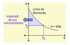
The market determines the price at which a product is sold. The point of intersection of the demand curve and the supply curve for a product gives the equilibrium price. At the equilibrium price, consumers will buy the same amount of product that manufacturers want to sell. However, some consumers will agree to spend more on an item than the equilibrium price. The total of the differences between the equilibrium price of the item and the higher prices that all these people accept to pay. Basically considered as a saving of those people and is called the consumer surplus.
The area under the demand curve is the total amount that consumers are willing to pay for q 0 items. The shaded area under the line y = p 0 shows the total amount that consumers actually spent on the price p 0 balance. The area between the curve and the straight line represents the consumer surplus.
Formula and Derivation
The consumer surplus is given by the area between the curves p = d (q) and p = p 0 then its value may encounter a definite integral as follows:

The demand curve is given by law d (x) = 50 – 0,06x 2 . Find the surplus or profit of the consumers if the level of sale amounts to twenty units.
As the number of units is 20, its price rises p = d (20) = 50 – 0.06 20 2 = 26.
Solving the integral, the profit of consumer’s results:
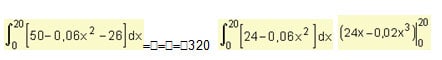
The consumer gain is $ 320 if the level of sales is twenty units.
In the same way if some manufacturers were willing to provide a product at a lower price than the price p 0 of balance. So the total differences between the equilibrium price and the lowest prices at which manufacturers sell the product is considered. Actually as an additional input for manufacturers and is called the producers’ surplus.

The total area under the supply curve between q = 0 and q = q 0 is the total minimum amount that manufacturers are willing to get from the sale of q 0 items. The total area under the line p = p 0 is the amount actually obtained. So the difference between these two areas, the surplus of producers, is also given by a definite integral.
If s (q) is a function of supply with price p 0 balance and offer q 0 of balance, then
![]()
It is known that the supply curve for a product is s (x) = . Find the profit of the
![]()

Example
Calculate excess supply and excess demand for given demand and supply curves.
Demand function: p 1 (q) = 1000 – 0.4 q 2 . Supply function: p 2 (q) = 42q
The excess supply and demand are represented by the areas shown in the graph:

Supply matches demand (q 0 , p 0 ), i.e. ,:
p 1 (q) = p 2 (q) Þ 1000 – 0,4q 2 = 42q Þ – 0,4q 2 – 42q + 1000 = 0 Þ
q 1 = – 125 Ù q 2 = 20
Since the values of the abscissa corresponds to the number of items offered or demanded, q 0 = 20. Therefore, p 0 = 840.
The excess demand or consumer surplus is the region between p 1 (q) and the line p = 840, between 0 and 20, i.e.

The demand surplus amounts to $ 2133.33
The excess supply is the region between the lines p = 840 and p = 42q between 0 and 20 that is:
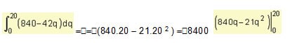
Offer surplus reaches $ 8400.
Marginal Analysis
The derivative and consequently the whole, have applications in business and economics in the construction of the marginal rates .
It is important to the economists this work with the marginal analysis because it allows calculating the point of maximization of utilities.
The marginal analysis examines the incremental effects on profitability. If a firm is producing a certain number of units per year, the marginal analysis addresses the effect that is reflected in the utility if an additional unit is produced and sold.
In order for this method to be applied to profit maximization, the following conditions must be met:
- It should be possible to identify separately the functions of total income and total cost.
- The functions of income and cost must be formulated in terms of the level of production or the number of units produced and sold.
We give some important definitions for our work:
Marginal Cost
It is the extra cost you get to produce and sell one more unit of a product or service.
It can also be defined as the limit value of the average cost per extra item when this number of extra items tends to zero.
We can think of marginal cost as the average cost per extra item when a very small change in quantity is made.
We must take into account that if c (x) is the cost function, the average cost of producing x items is the total cost divided by the number of items produced.
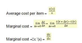
The marginal cost measures the rate at which the cost increases with respect to the increase of the quantity produced.
Marginal Revenue
It is the additional income that is achieved by selling one more unit of a product or service.
For a total income function r (x), the derivative r ‘(x) represents the instantaneous rate of change in total income with a change in the number of units sold. We can say that the marginal revenue represents the additional inputs of one company per additional item sold when a very small increase occurs in the number of items sold. It represents the rate at which income grows in relation to the increase in sales volume.
Marginal Utility
It is that gets a company is given by the difference between their income and costs. If the input function is r (x) when x items are sold and if the cost function is c (x) when these same articles are produced, the utility p (x) obtained by producing and selling x items is given by p x) = r (x) – c (x).
The derivative p ‘(x) is called marginal utility and represents the utility per item if production suffers a small increase.
Solve the following issues and check the answers.
A marginal cost function is defined by c ‘(x) = 3x 2 + 8x + 4 and the fixed cost is $ 6. Determine the corresponding total cost function.
Answer: c (x) = x 3 + 4x 2 + 4x + 6
For a particular item, the marginal revenue function is i ‘(x) = 15 – 4x. If x units are demanded when the price per unit is p pesos:
- Determine the total revenue function.
- Determine the demand equation.
Answers: a) i (x) = 15x – 2x 2 b) p (x) = 15 – 2x
We assume that during the first five years that a product was put on the market the f (x) function describes the sales ratio when x years passed since the product was first introduced on the market.
Example
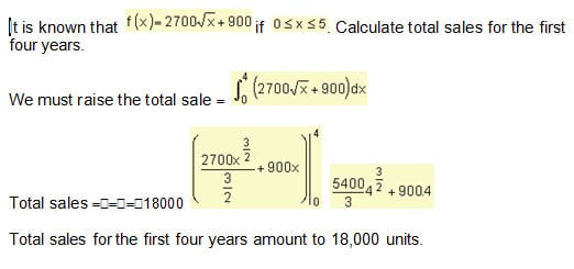
The purchase of a new machine is expected to generate savings in operating costs. When the machine has x years of use the savings ratio is f (x) pesos a year where f (x) = 1000 + 5000x.
- How much will save on operating costs during the first six years?
- If the machine was purchased at $ 67500 How long will the machine pay for itself?
- To achieve the savings during the first six years calculate
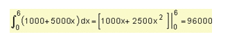
After six years the savings amount to $ 96000
- Since the purchase price is $ 67500, the number of years of use required to pay the machine alone is n, then
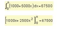
1000n + 2500 n 2 = 67500 Þ 2500 n 2 + 1000n – 67500 = 0
5 n 2 + 2n – 135 = 0
We found values of n and applying the resolving is n 1 = – 5.4 (impossible for our problem) and also n 2 = 5.
It will take 5 years for the machine to pay for itself.
When economists claim market equilibrium is allocatively efficient, they’re referring to this. It is impossible to increase consumer surplus without reducing producer surplus at the productive level of production, and it is also impossible to increase producer surplus without reducing consumer surplus.

Hello everyone! This is Richard Daniels, a full-time passionate researcher & blogger. He holds a Ph.D. degree in Economics. He loves to write about economics, e-commerce, and business-related topics for students to assist them in their studies. That's the sole purpose of Business Study Notes.
Love my efforts? Don't forget to share this blog.


